1. 前言
比较转录组作为生信分析中最常规的分析,底层逻辑是通过基因的表达量,筛选差异基因,随后进行下游的富集分析。也可以通过表达量矩阵进行时序分析和WGCNA分析。那么,这种分析模式可不可以用在其他分析中呢,我个人认为是可以的。因此今天就把这套流程应用在宏基因组分析中,用基因的丰度代替基因的表达量,来进行一些分析。
2. 分析
2.1 DESeq2差异分析
通过基因的丰度数据进行差异分析,需要注释的是,丰度要是原始的Count,不能是标准化后的TMP和FPKM。这一步的输入文件是(1)基因丰度(2)样品分组信息
| sample | condition |
|---|---|
| J1 | J |
| J2 | J |
| J3 | J |
| J4 | J |
| F1 | F |
| F2 | F |
| F3 | F |
| F4 | F |
| GeneID | F2 | J1 | J4 | J3 | J2 | F4 | F1 | F3 | Total |
|---|---|---|---|---|---|---|---|---|---|
| J2_k97_737169_1 | 298 | 318 | 4 | 2 | 8 | 90 | 20 | 30 | 770 |
| J2_k97_737170_1 | 0 | 0 | 2 | 2 | 6 | 0 | 0 | 0 | 10 |
| J2_k97_105311_1 | 0 | 0 | 2 | 0 | 2 | 0 | 0 | 0 | 4 |
| J2_k97_1684952_1 | 0 | 0 | 8 | 0 | 6 | 0 | 0 | 0 | 14 |
| J2_k97_1369023_1 | 0 | 0 | 2 | 0 | 2 | 0 | 0 | 2 | 6 |
| J2_k97_1369023_2 | 0 | 0 | 2 | 4 | 10 | 0 | 0 | 2 | 18 |
| J2_k97_631861_1 | 0 | 0 | 0 | 2 | 0 | 0 | 0 | 0 | 2 |
# --- 1. 设置工作环境 ---

# 加载所需的R包
# 如果您尚未安装这些包,请先运行 install.packages("包名") 进行安装
# 例如: install.packages("DESeq2")
suppressPackageStartupMessages({
  library(DESeq2)
  library(readr)
  library(dplyr)
})

# --- 2. 设置输入和输出文件 ---
# 请根据您的文件位置修改以下路径

# 设置原始基因count矩阵文件的路径 (例如: "data/reads_number.xls")
# 文件应为制表符分隔,第一列为基因ID,后续列为样本的count值。
count_file <- "reads_number.xls"

# 设置样本信息文件的路径 (例如: "data/sample_info.csv")
# 文件应为逗号分隔,包含两列: "sample" (样本名称) 和 "condition" (分组信息)。
sample_info_file <- "sample_info.csv"

# 设置输出文件的前缀 (例如: "results/deseq2_output")
# 脚本将生成一个名为 <output_prefix>_diff_expression.csv 的结果文件。
output_prefix <- "deseq2_results"


# --- 3. 读取并预处理数据 ---

# 读取原始基因count矩阵
# 假设文件是制表符分隔的,第一列是基因ID
cat(paste0("正在读取count文件: ", count_file, "\n"))
count_data <- read.delim(count_file, row.names = 1, sep = "\t", check.names = FALSE)

# 删除count数据中的最后一列
# 原始脚本位置: /home/majunpeng/sda2/Lishuyan_Kuozangzi_sequence/Metagenome/Gemini/deseq2_analysis_rstudio_1.R
count_data <- count_data[, -ncol(count_data)]

# 读取样本信息文件
# 假设文件是逗号分隔的
cat(paste0("正在读取样本信息文件: ", sample_info_file, "\n"))
sample_info <- read_csv(sample_info_file, show_col_types = FALSE)

# 确保count数据是整数类型,DESeq2要求输入为整数
count_data <- round(count_data)

# 确保样本信息中的样本名称与count数据中的列名一致且顺序一致
# 筛选出在count数据中存在的样本
sample_info <- sample_info %>%
  filter(sample %in% colnames(count_data)) %>%
  arrange(match(sample, colnames(count_data))) # 按照count数据的列顺序排序

# 检查样本数量是否匹配
if (ncol(count_data) != nrow(sample_info)) {
  stop("错误: count数据中的样本列数与样本信息文件中的样本行数不匹配。请检查您的输入文件。\n")
}

# 确保count数据的列名和sample_info的sample列顺序一致
count_data <- count_data[, sample_info$sample]

# 将condition列转换为因子,并设置比较组和对照组
# DESeq2默认按字母顺序确定对照组,例如'F'和'J'中,'F'会成为对照组。
# 为了明确指定对照组,我们使用relevel()函数。
# 这里我们将'J'设置为对照组(reference level)。
unique_conditions <- unique(sample_info$condition)
if (length(unique_conditions) < 2) {
  stop("错误: 样本信息中至少需要两个不同的条件才能进行差异表达分析。\n")
}
# 假设您想比较 F组 vs J组,J组是对照组
sample_info$condition <- factor(sample_info$condition)
sample_info$condition <- relevel(sample_info$condition, ref = "F")


# --- 4. 构建DESeqDataSet对象 ---

# 创建DESeqDataSet对象
# design公式指定了如何进行差异分析,这里是根据condition进行比较
dds <- DESeqDataSetFromMatrix(countData = count_data,
                              colData = sample_info,
                              design = ~ condition)

# 过滤低表达基因 (可选,但推荐)
# 过滤掉在所有样本中count总和过低的基因,以减少计算量和提高统计功效
# 这里保留那些在至少一个样本中count大于等于10的基因
keep <- rowSums(counts(dds) >= 10) >= 1
dds <- dds[keep,]

# --- 5. 运行DESeq2核心分析 ---

cat("正在运行DESeq2差异表达分析...\n")
dds <- DESeq(dds)

# --- 6. 提取和保存结果 ---

# 提取差异表达结果
# resultsNames(dds) 可以查看所有可用的比较名称
# 默认情况下,它会比较处理组与您设定的对照组
res <- results(dds)

# 您也可以使用 contrast 参数明确指定比较,例如比较'F'组相对于'J'组的差异
# res <- results(dds, contrast = c("condition", "F", "J"))

# 对结果进行排序 (例如,按调整后的p值(padj)从小到大排序)
res_ordered <- res[order(res$padj),]

# 将结果转换为数据框
res_df <- as.data.frame(res_ordered)

# 添加基因ID列
res_df <- tibble::rownames_to_column(res_df, var = "gene_id")

# 保存结果到CSV文件
output_file <- paste0(output_prefix, "_diff_expression.csv")
cat(paste0("正在保存差异表达结果到: ", output_file, "\n"))
write_csv(res_df, output_file)

cat("DESeq2分析完成!\n")
最后,我们就一定拿到了差异分析的结果,接下来我们以P值小于等于0.05,Log2FC的绝对值大于等于1.5进行差异基因的筛选。
| gene_id | baseMean | log2FoldChange | lfcSE | stat | pvalue | padj |
|---|---|---|---|---|---|---|
| J3_k97_1869542_48 | 719.9416276 | 26.53634325 | 2.584192382 | 10.26871816 | 9.75E-25 | 1.10E-18 |
| J3_k97_1869542_49 | 505.5442894 | 26.1670583 | 2.571273542 | 10.17669177 | 2.52E-24 | 1.42E-18 |
| J3_k97_1869542_3 | 502.7114513 | 26.08115486 | 2.581835499 | 10.101788 | 5.42E-24 | 1.53E-18 |
| J3_k97_1869542_47 | 495.3948077 | 25.74264487 | 2.546306163 | 10.10979954 | 5.00E-24 | 1.53E-18 |
| J3_k97_1869542_33 | 623.4655207 | 26.26834756 | 2.607327384 | 10.0748175 | 7.14E-24 | 1.61E-18 |
| J3_k97_1869542_67 | 311.7707339 | 25.4921083 | 2.547029189 | 10.00856543 | 1.40E-23 | 2.63E-18 |
| J3_k97_1869542_32 | 554.8218292 | 26.2904605 | 2.632630124 | 9.986385957 | 1.75E-23 | 2.82E-18 |
| J3_k97_1869542_14 | 377.7311327 | 25.44960062 | 2.552398401 | 9.970857455 | 2.04E-23 | 2.89E-18 |
| J3_k97_1869542_8 | 404.1818614 | 25.85406933 | 2.612079894 | 9.89788612 | 4.25E-23 | 4.23E-18 |
2.2 富集分析
富集分析主要分为两部分,常规的KEGG和GO富集分析和GSEA富集分析。第一步就是要通过Eggnog的注释结果构建一个Orgdb库。
					emapper
Rscript /pub/software/emcp/emapperx.R out.emapper.annotations proteins.fa
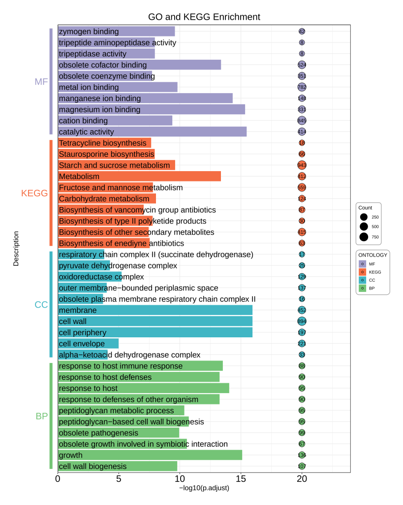
随后进行常规的KEGG和GO富集分析,这一步我使用的是TBtools,在这里就不详细解释怎么用了,请自行搜索学习。完成富集分析后,按照下面的输入文件格式简单的整理一下,下面的是一个KEGG和GO富集可视化的代码。
| ONTOLOGY | Description | p.adjust | Count |
|---|---|---|---|
| KEGG | Metabolism | 4.30E-14 | 412 |
| KEGG | Starch and sucrose metabolism | 2.42E-10 | 943 |
| KEGG | Carbohydrate metabolism | 8.78E-09 | 124 |
| KEGG | Staurosporine biosynthesis | 1.11E-08 | 66 |
| KEGG | Fructose and mannose metabolism | 1.56E-08 | 559 |
| KEGG | Biosynthesis of type II polyketide products | 1.68E-08 | 30 |
| KEGG | Tetracycline biosynthesis | 2.21E-08 | 18 |
| KEGG | Biosynthesis of enediyne antibiotics | 2.91E-08 | 63 |
| KEGG | Biosynthesis of other secondary metabolites | 3.49E-08 | 415 |
| KEGG | Biosynthesis of vancomycin group antibiotics | 9.06E-08 | 87 |
| MF | catalytic activity | 3.33E-16 | 414 |
| MF | magnesium ion binding | 4.44E-16 | 331 |
| MF | manganese ion binding | 4.66E-15 | 148 |
| MF | obsolete cofactor binding | 4.13E-14 | 524 |
| MF | metal ion binding | 1.55E-10 | 782 |
| MF | zymogen binding | 2.49E-10 | 42 |
| MF | cation binding | 4.05E-10 | 845 |
| MF | tripeptide aminopeptidase activity | 1.10E-08 | 8 |
| MF | tripeptidase activity | 1.10E-08 | 8 |
| MF | obsolete coenzyme binding | 1.84E-08 | 351 |
| CC | cell periphery | 1.11E-16 | 197 |
| CC | cell wall | 1.11E-16 | 894 |
| CC | membrane | 1.11E-16 | 452 |
| CC | oxidoreductase complex | 5.77E-06 | 129 |
| CC | cell envelope | 1.03E-05 | 221 |
| CC | pyruvate dehydrogenase complex | 5.25E-05 | 25 |
| CC | alpha-ketoacid dehydrogenase complex | 8.13E-05 | 33 |
| CC | outer membrane-bounded periplasmic space | 9.59E-05 | 137 |
| CC | respiratory chain complex II (succinate dehydrogenase) | 0.000151272 | 17 |
| CC | obsolete plasma membrane respiratory chain complex II | 0.000192509 | 16 |
| BP | growth | 7.77E-16 | 136 |
| BP | response to host | 8.88E-15 | 95 |
| BP | response to host immune response | 2.95E-14 | 88 |
| BP | response to defenses of other organism | 5.51E-14 | 90 |
| BP | response to host defenses | 5.51E-14 | 90 |
| BP | peptidoglycan-based cell wall biogenesis | 1.84E-11 | 95 |
| BP | obsolete growth involved in symbiotic interaction | 2.59E-11 | 67 |
| BP | peptidoglycan metabolic process | 4.20E-11 | 95 |
| BP | obsolete pathogenesis | 1.12E-10 | 99 |
| BP | cell wall biogenesis | 1.61E-10 | 107 |
					rm(list = ls())


####----load R Package----####
library(tidyverse)
library(ggh4x)
library(ggfun)
library(clusterProfiler)
library(org.Hs.eg.db)

####----load Result----####

plot_df <- read.csv("KEGG_GO富集绘图.csv")
####----Plot----####
plot <- plot_df %>%
  ggplot() +
  geom_bar(aes(x = -log10(p.adjust), y = interaction(Description, ONTOLOGY), fill = ONTOLOGY), stat = "identity") +
  geom_text(aes(x = 0.1, y = interaction(Description, ONTOLOGY), label = Description), size = 6, hjust = "left", color = "#000000") +
  geom_point(aes(x = 20, y = interaction(Description, ONTOLOGY), size = Count, fill = ONTOLOGY), shape = 21) +
  geom_text(aes(x = 20, y = interaction(Description, ONTOLOGY), label = Count)) +
  scale_x_continuous(expand = expansion(mult = c(0, 0.2))) +
  scale_fill_manual(values = c("#74c476", "#41b6c4", "#f46d43", "#9e9ac8")) +
  scale_size(range = c(5, 8.5),
             guide = guide_legend(override.aes = list(fill = "#000000"))) +
  guides(y = "axis_nested",
         fill = guide_legend(reverse = T)) +
  labs(x = "-log10(p.adjust)", y = "Description") +
  ggtitle(label = "GO and KEGG Enrichment") +
  theme_bw() +
  theme(
    ggh4x.axis.nestline.y = element_line(size = 3, color = c("#74c476", "#41b6c4", "#f46d43", "#9e9ac8")),
    ggh4x.axis.nesttext.y = element_text(colour = c("#74c476", "#41b6c4", "#f46d43", "#9e9ac8")),
    legend.background = element_roundrect(color = "#969696"),
    panel.border = element_rect(linewidth = 1),
    plot.margin = margin(t = 1, r = 1, b = 1, l = 1, unit = "cm"),
    axis.text = element_text(color = "#000000", size = 20),
    axis.text.y = element_text(color = rep(c("#41ae76", "#225ea8", "#fc4e2a", "#88419d"), each = 10)),
    axis.text.y.left = element_blank(),
    axis.ticks.length.y.left = unit(10, "pt"),
    axis.ticks.y.left = element_line(color = NA),
    axis.title = element_text(color = "#000000", size = 15),
    plot.title = element_text(color = "#000000", size = 20, hjust = 0.5)
  )

plot

ggsave(filename = "GO_KEGG_Lishuyan.pdf",
       plot = plot,
       height = 15,
       width = 12)

####----sessionInfo----####
sessionInfo()
| gene_id | log2FoldChange |
|---|---|
| J3_k97_1869542_48_1 | 26.53634325 |
| J3_k97_1869542_32_1 | 26.2904605 |
| J3_k97_1869542_33_1 | 26.26834756 |
| J3_k97_1869542_49_1 | 26.1670583 |
| J3_k97_1869542_3_1 | 26.08115486 |
| J3_k97_1869542_45_1 | 25.94958501 |
| J3_k97_1869542_8_1 | 25.85406933 |
| J3_k97_1869542_23_1 | 25.82508916 |
| J3_k97_1869542_47_1 | 25.74264487 |
| J3_k97_1869542_75_1 | 25.69997138 |
| J3_k97_1869542_60_1 | 25.6210279 |
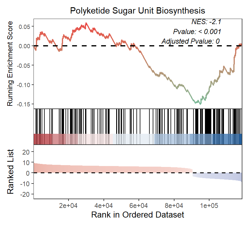
接下来进行GSEA富集分析,同样,需要按照下面的格式整理的一个输入文件,包含基因ID和Log2FC值信息。
					library(magrittr)
library(readr)
library(clusterProfiler)
library(tidyr)
library(tibble)
library(stringr)
library(GseaVis)


get_path2name <- function(){
  keggpathid2name.df <- clusterProfiler:::kegg_list("pathway")
  keggpathid2name.df[,1] %<>% gsub("path:map", "", .)
  colnames(keggpathid2name.df) <- c("path_id","path_name")
  return(keggpathid2name.df)
}
pathway2name <- get_path2name()
pathway2name$path_id <- gsub("map", "", pathway2name$path_id, ignore.case = TRUE)

emapper <- read_delim("../EGGNOG.emapper.annotations",
                      "\t", escape_double = FALSE, col_names = FALSE,
                      comment = "#", trim_ws = TRUE) %>%
  dplyr::select(GID = X1,
                COG = X7,
                Gene_Name = X8,
                Gene_Symbol = X9,
                GO = X10,
                KO = X12,
                Pathway = X13
  )

pathway2gene <- dplyr::select(emapper, Pathway, GID) %>%
  separate_rows(Pathway, sep = ',', convert = F) %>%
  filter(str_detect(Pathway, 'ko')) %>%
  mutate(Pathway = str_remove(Pathway, 'ko'))


gene_data <- read.csv("差异基因表达量.csv")

geneList <- setNames(gene_data$log2FoldChange, gene_data$gene_id)

geneList <- sort(geneList, decreasing = TRUE)

head(geneList)

ekp2 = GSEA(
  geneList,
  TERM2GENE = pathway2gene,
  TERM2NAME = pathway2name,
  minGSSize = 10,
  maxGSSize = 500,
  pvalueCutoff = 0.05)

ekp2_df <- as.data.frame(ekp2)
write.csv(as.data.frame(ekp2), "GSEA_analysis_KEGG.csv", row.names = FALSE)

gseaNb(object = ekp2,
       geneSetID = '00523',
       addPval = T,
       rankSeq = 20000)

GSEA_fig <- gseaNb(object = ekp2,
       geneSetID = c('00523',"01059", "00404"),
       addPval = T,
       rankSeq = 20000,
       pvalX = 0.15,pvalY = 0.15)

ggsave("GSEA.pdf", GSEA_fig, width = 8, height = 6, dpi = 300)
2.3 WGCNA分析
同样WGCNA也可以做,找到和某个ASV相关性最高的基因。
					library(WGCNA)
library(tidyverse)

# 读取基因丰度文件
gene_exp <- read.csv(file = '差异基因_TPM.csv',
                     row.names = 1)

# 读取扩增子ASV风度文件
sample_info <- read.table(file = 'ASV_Count.txt',
                        row.names = 1, header = TRUE )

{
  # 转置
  datExpr0 <- t(gene_exp)

  # 缺失数据及无波动数据过滤
  gsg <- goodSamplesGenes(
    datExpr0,
    minFraction = 1/2 #基因的缺失数据比例阈值
  )
  datExpr <- datExpr0[gsg$goodSamples, gsg$goodGenes]

  # 通过聚类,查看是否有明显异常样本, 如果有需要剔除掉
  plot(hclust(dist(datExpr)),
       cex.lab = 1.5,
       cex.axis = 1.5,
       cex.main = 2)


  # 如果剩余基因仍然太多(如 5 到10万条),
  ##而电脑配置内存不够,可以进一步过滤掉
  ##波动小的基因。不要只用差异基因做。
  # library(genefilter)
  # var_gene_exp <- varFilter(
  #   as.matrix(t(datExpr)),
  #   var.func = IQR,
  #   var.cutoff = 0.5, # 实际项目中设置 0.5 以下
  #   filterByQuantile = TRUE)
  #
  # datExpr <- t(var_gene_exp)
  datExpr[1:4,1:4]
}

{
  datTraits <- sample_info
}

{
  library(WGCNA)
  # 多线程
  enableWGCNAThreads(nThreads = 80)
  ## disableWGCNAThreads()

  # 通过对 power 的多次迭代,确定最佳 power
  sft <- pickSoftThreshold(
    datExpr,
    powerVector = 1:20, # 尝试 1 到 20
    networkType = "unsigned"
  )
}

{
  # 画图
  library(ggplot2)
  library(ggrepel)
  library(cowplot)
  library(ggthemes)

  fig_power1 <- ggplot(data = sft$fitIndices,
                       aes(x = Power,
                           y = SFT.R.sq)) +
    geom_point(color = 'red') +
    geom_text_repel(aes(label = Power)) +
    geom_hline(aes(yintercept = 0.85), color = 'red') +
    labs(title = 'Scale independence',
         x = 'Soft Threshold (power)',
         y = 'Scale Free Topology Model Fit,signed R^2') +
    theme_few() +
    theme(plot.title = element_text(hjust = 0.5))

  fig_power2 <- ggplot(data = sft$fitIndices,
                       aes(x = Power,
                           y = mean.k.)) +
    geom_point(color = 'red') +
    geom_text_repel(aes(label = Power)) +
    labs(title = 'Mean connectivity',
         x = 'Soft Threshold (power)',
         y = 'Mean Connectivity') +
    theme_few()+
    theme(plot.title = element_text(hjust = 0.5))

  plot_grid(fig_power1, fig_power2)
}

{
  net <- blockwiseModules(
    # 0.输入数据
    datExpr,

    # 1. 计算相关系数
    corType = "pearson", # 相关系数算法,pearson|bicor

    # 2. 计算邻接矩阵
    power = 6, # 前面得到的 soft power
    networkType = "unsigned", # unsigned | signed | signed hybrid

    # 3. 计算 TOM 矩阵
    TOMType = "unsigned", # none | unsigned | signed
    saveTOMs = TRUE,
    saveTOMFileBase = "blockwiseTOM",

    # 4. 聚类并划分模块
    deepSplit = 2, # 0|1|2|3|4, 值越大得到的模块就越多越小
    minModuleSize = 30,

    # 5. 合并相似模块
    ## 5.1 计算模块特征向量(module eigengenes, MEs),即 PC1
    ## 5.2 计算 MEs 与 datTrait 之间的相关性
    ## 5.3 对距离小于 mergeCutHeight (1-cor)的模块进行合并
    mergeCutHeight = 0.25,

    # 其他参数
    numericLabels = FALSE, # 以数字命名模块
    nThreads = 0, # 0 则使用所有可用线程
    maxBlockSize = 200000 # 需要大于基因的数目
  )
  # 查看每个模块包含基因数目
  table(net$colors)
}

{
  # 同时绘制聚类图和模块颜色
  plotDendroAndColors(
    dendro = net$dendrograms[[1]],
    colors = net$colors,
    groupLabels = "Module colors",
    dendroLabels = FALSE,
    addGuide = TRUE)
}

{
  # 计算相关性
  moduleTraitCor <- cor(
    net$MEs,
    datTraits,
    use = "p",
    method = 'spearman' # 注意相关系数计算方式
  )

  # 计算 Pvalue
  moduleTraitPvalue <- corPvalueStudent(
    moduleTraitCor,
    nrow(datExpr))
}

{
  # 相关性 heatmap
  sizeGrWindow(10,6)

  # 连接相关性和 pvalue
  textMatrix <- paste(signif(moduleTraitCor, 2), "\n(",
                      signif(moduleTraitPvalue, 1), ")", sep = "");
  dim(textMatrix) <- dim(moduleTraitCor)


  # heatmap 画图
  par(mar = c(6, 8.5, 3, 3))
  labeledHeatmap(Matrix = moduleTraitCor,
                 xLabels = names(datTraits),
                 yLabels = names(net$MEs),
                 ySymbols = names(net$MEs),
                 colorLabels = FALSE,
                 colors = blueWhiteRed(50),
                 textMatrix = textMatrix,
                 setStdMargins = FALSE,
                 cex.text = 0.5,
                 zlim = c(-1,1),
                 main = paste("Module-trait relationships"))
}

{
  # 创建简化版的 WGCNA 结果(不需要 gene_info)
  wgcna_result <- data.frame(
    gene_id = names(net$colors),
    module = net$colors,
    stringsAsFactors = FALSE
  )

  # 查看结果
  head(wgcna_result)
  table(wgcna_result$module)
}

{
  # 需要导出的模块
  my_modules <- c('brown')

  # 提取该模块的表达矩阵
  m_wgcna_result <- filter(wgcna_result, module %in% my_modules)
  m_datExpr <- datExpr[, m_wgcna_result$gene_id]

  # 计算该模块的 TOM 矩阵
  m_TOM <- TOMsimilarityFromExpr(
    m_datExpr,
    power = 6,
    networkType = "unsigned",
    TOMType = "unsigned")

  dimnames(m_TOM) <- list(colnames(m_datExpr), colnames(m_datExpr))

  # 导出 Cytoscape 输入文件
  cyt <- exportNetworkToCytoscape(
    m_TOM,
    edgeFile = "CytoscapeInput-network.txt",
    weighted = TRUE,
    threshold = 0.2)
}
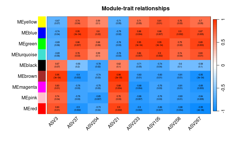
通过每个模块上方显著性和下方的p值来筛选显著的模块,比如和ASV呈现正相关的为brown,负相关的为blue。